
The image processing produces a 1 bit image (B&W) of 240x144 pixels. The next step is to take this image and convert it into movements for the motors.
The way this is done is governed largely by the design of the Etch-A-Sketch — any drawing must be made in one, single, continuous line. To draw any of the dark pixels in our 100x60 image, we must drive the pointer over to that location, covering only other regions of the image that are also supposed to be dark.
The good news is that the edge-finding algorithm produces an 1-pixel width line, and if enabled the hash-filling is also 1 pixel thick. The trick then is simply to find a ‘route’ through the image that covers all of the pixels. This lends itself nicely to graph theory and in Python in particular the networkx library.
What is a graph?
A graph is a network made up of a number of points (or nodes) which are connected to nodes through links (or edges). An edge is defined by the two nodes that it connects, and any given node can have multiple connections to other nodes.
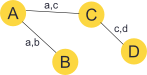
We are using undirected graphs, where edges are bi-directional. That is a link from A to B is also a link from B to A.
The pixel drawing can be represented as a graph where a dark pixel is a node_and the relationship between it and an _adjacent pixel is represented as an edge. This adjacent pixel has edges representing connections to its neighbours, and so on.
![]()
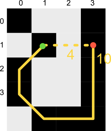
Using this representation we can quickly find a traversable route from our current pixel to any connected pixel in the image as a series of single pixel steps. In the above image for example, our route from 0,0 to 2,3 would take us through 1,1 and 1,2.
There is some memory overhead for using this approach, but networkx is efficient and fast enough for a network this small.
Building a graph
The process for building a graph from an input image is shown below. The process is as follows.
- Iterate through all pixels in the image (order is unimportant)
- Check the adjacent pixels in the directions up-right, right, down-right and down
- For each adjacent pixel which is filled, add an edge from the current pixel to it —
networkxautomatically creates the nodes.
![]()
Note that we only need to check 4 of the 8 directions (we can ignore down-left, left, up-left and up) as the connections we form are bi-directional.
import networkx as nx

def build_graph(image):

    data = np.array(image).T
    width, height = data.shape

    # Build a network adjacency graph for black pixels in the image.
    G = nx.Graph()
        for x in range(0, width):
        for y in range(0, height):
            curr = (x, y)
            if data[curr]: # white = 255
                continue

            if x < width - 1:
                right = (x + 1, y)
                if not data[right]:
                    G.add_edge(curr, right)

                if y > 0:
                    rup = (x + 1, y - 1)
                    if not data[rup]:
                        G.add_edge(curr, rup)

                if y < height - 1:
                    rdown = (x + 1, y + 1)
                    if not data[rdown]:
                        G.add_edge(curr, rdown)

            if y < height - 1:
                down  = (x, y + 1)
                if not data[down]:
                    G.add_edge(curr, down)

    return G
The result of this processing is a graph containing subgraphs of pixels which are connected through other adjacent pixels. There may be only 1 subgraph, but there may also be many more. In the next step we'll process the graph further to connect these subgraphs into one.
Linking lines
In order to be able to draw the image on an Etch-A-Sketch we need to ensure the connectivity of all pixels in the picture. While shader fills work to produce connected graphs complex areas of the image turn into a bundle of noise — and it takes ages to draw all these parts.
To speed up drawing I also implemented an simpler method which just finds the shortest straight-line joins between all subgraphs of the image. This loses the shading and adds some extra lines, but makes for much faster snaps.
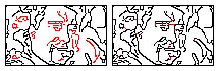
To do this we iterate each graph's nodes in turn and find the shortest lines we can draw to connect the current graph with any other graph. We repeat this until there is only a single graph left. The below image shows this linking approach used on a poorly connected graph.The first panel shows the main graph in black and all unconnected subgraphs shown in red. The second panel shows the linker lines (in red) after all subgraphs have been connected.
The final optimisation is to increase the connectivity of the graph. Any gaps less than SHORT_LINK_LEN in distance (euclidean) are stored. If, after combining all graphs, the distance between these points is greater than SHORT_LINK_THRESHOLD we connect them by adding shortcuts across the gaps.
The processing code for adding subgraph linker lines and the connectivity additions is below.
def connect_graph(G):
    """
    Add additional edges to the provided graph until all edges are connected.
    Performed iteratively, connecting each subsequent graph to the the largest
    """

    graphs = list(nx.connected_component_subgraphs(G))

    if len(graphs) > 1:
        combinations = itertools.combinations(graphs, 2)
        shortest = {}
        links = []

        for g0, g1 in combinations:

            # For each node in the graph, compare vs. all nodes in the giant-list. The
            # difference x,y must be 1:1 (diagonal), then find the shortest + link.
            g_ix = (g0, g1)
            for n1 in g1.nodes:
                for n0 in g0.nodes:
                    d = euclidean_distance_45deg(n1, n0)
                    if d:
                        link = d, n0, n1

                        # Find global short links
                        if (shortest.get(g_ix) is None or d < shortest.get(g_ix)[0]):
                            shortest[g_ix] = link

                        if d < SHORT_LINK_LEN:
                            # Sub-graph link which is short, can be used to shortcut.
                            links.append(link)

        # We have a list of shortest graph-graph connections. We want to find the shortest connections
        # neccessary to connect *all* graphs. If we connect A-B and B-C then A-B-C are all connected.
        # Start from the largest graph and the shortest links and work backwards.
        shortlinks = sorted(shortest.items(), key=lambda x: x[1][0])  # Sort by link data x[1], first part [0] = d
        connected = [max(graphs, key=len)]  # Our current connected graphs

        while len(connected) < len(graphs):
            shortest = None
            # Find the shortest link for any graph in connected to any graph that isn't.
            for (g0, g1), link in shortlinks:
                d, n0, n1 = link
                if (g0 in connected and g1 not in connected) and (shortest is None or d < shortest[1][0]):
                    shortest = g1, link

                if (g1 in connected and g0 not in connected) and (shortest is None or d < shortest[1][0]):
                    shortest = g0, link

            if shortest:
                g, (d, n0, n1) = shortest
                G.add_edge(n0, n1, weight=d)
                connected.append(g)

        # Use detected short links to minimise the path lengths
        for link in sorted(links, key=lambda x: x[0]):
            d, n0, n1 = link
            if shortest_path_length(G, n0, n1, weight='weight') >= SHORT_LINK_THRESHOLD:
                G.add_edge(n0, n1, weight=d)

    return G
These links are added as edges without intermediate nodes. This means that the lines will not be required only drawn if needed.
We’re ranking the connections using Euclidean distance (a fancy way of saying “as the crow flies”) but only allowing 45/90 degree angles (8 compass points) because of the limitations in the plotter code.
def euclidean_distance_45deg(a, b):
    """
    Return the euclidean distance between two points if they are on one of the 45 degree
    compass points. For any other angles return None.
    """
    xd, yd = (a[0]-b[0]), (a[1]-b[1])
    if (
        abs(xd) == abs(yd) or xd == 0 or yd == 0
    ):
        return math.sqrt( (xd)**2 + (yd)**2 )
The image below shows the original unconnected graph (left) and with linker lines (middle) as before, with the right panel showing (in green) the connectivity additions.
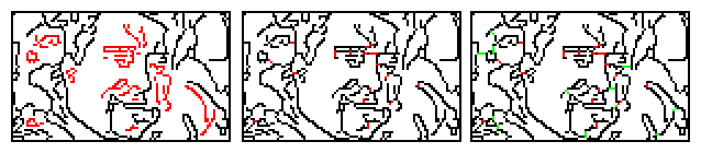
This method shortens the draw time considerably at the expense of extending the processing time. It would be possible to postpone this optimization to the drawing phase, adding the bridges in the background so the delay is less noticeable.
Calculating moves from the graph
We don’t optimise the route through the graph with a traveling-salesman like algorithm, so the resulting path can be quite daft.
from networkx.algorithms.shortest_paths.generic import shortest_path, shortest_path_length

def calculate_moves(G):
    """
    Calculate the moves neccessary to draw the provided graph.
    """

    # Take a copy of the input graphs nodes, so we can remove nodes as we go without affecting pathfinding.
    rgiant = list(Gc.nodes)

    n = 0
    start = (0, 0)

    def distance(n):
        # Note that start is modified by the loop.
        return math.sqrt(
            (n[0]-start[0])**2 +
            (n[1]-start[1])**2
        )

    while rgiant:
        n += 1
        dnode = min(rgiant, key=distance)
        rgiant.remove(dnode)

        path = shortest_path(G, start, dnode, weight='weight')
        last_node = start

        # Traverse the path, yield all the steps required to get there.
        for node in path[1:]:
            # Yield this step to draw it (x & y can be > 1), may require multiple steps.
            yield (node[0] - last_node[0], node[1] - last_node[1])

            # Keep reference of where we've been for later, increase weight to discourage re-drawing.
            G.edges[(node, last_node)]['weight'] = G.edges[(node, last_node)].get('weight', 1) * 2
            last_node = node

        # Chop away to avoid redundant paths.
        rgiant = set(rgiant) - set(path)

        # Update to our new position
        start = dnode

    # Plot and yield final path to home (0,0).
    path = shortest_path(G, last_node, (0, 0), weight='weight')
    for node in path[1:]:
        # Yield this step to draw it (x & y can be > 1), may require multiple steps.
        yield (node[0] - last_node[0], node[1] - last_node[1])
        last_node = node
This move calculation is daft, I mean really daft. The only mechanism in place to optimize the drawing on the screen is the the following line.
G.edges[(node, last_node)].get('weight', 1) * 2
This adds a cost (exponential) of re-drawing over the same spot when there are other alternatives available. However, the algorithm doesn't optimize decisions at forks, so will for example often continue past isolated regions of the image, only to have to back-track later to draw them. If you want to play around with optimising this the place to do so is the lines:
    dnode = min(rgiant, key=distance)
    rgiant.remove(dnode)
This picks the 'next' node by simply looking for what is nearest. If there are two adjacent pixels both will be nearest and the selection will be random. You could try introducing tie-breaking logic, or another mechanism for choosing path independent of the pixel distance.
What's next
The calculate_moves generator function yields a series of 2-tuples giving x,y delta (differences) that the plotter pointed should move. The final step is to take these instructions can convert them to movement in the stepper motors.
![]()

To support developers in [[ countryRegion ]] I give a [[ localizedDiscount[couponCode] ]]% discount on all books and courses.
[[ activeDiscount.description ]] I'm giving a [[ activeDiscount.discount ]]% discount on all books and courses.